Implementing Gibbs Sampling in Python

Suppose we have a joint distribution \(P\) on multiple random variables which we can’t sample from directly. But we require the samples anyhow. One way to sample from it is Gibbs sampling. Where we know that sampling from \(P\) is hard, but sampling from the conditional distribution of one variable at a time conditioned on rest of the variables is simpler. And it’s possible because sampling from 1D distributions is simpler in general.

For keeping things simple, we will program Gibbs sampling for simple 2D Gaussian distribution. Albeit its simple to sample from multivariate Gaussian distribution, but we’ll assume that it’s not and hence we need to use some other method to sample from it, i.e., Gibbs sampling.

Let our original distribution for which we need to sample be \(P \sim \mathcal{N}(\boldsymbol{\mu}, \Sigma)\). Where, \(\boldsymbol{\mu} \in \mathbb{R}^2\) is the mean vector and \(\Sigma \in \mathbb{R}^{2\times 2}\) is the symmetric positive semi-definite covariance matrix. And each of the sample will be \(\mathbf{x} = [x_0, x_1]^T\).

For Gibbs sampling, we need to sample from the conditional of one variable, given the values of all other variables. So in our case, we need to sample from \(p(x_0\vert x_1)\) and \(p(x_1\vert x_0)\) to get one sample from our original distribution \(P\). So, our main sampler will contain two simple sampling from these conditional distributions:

def gibbs_sampler(initial_point, num_samples, ...):
    x_0 = initial_point[0]
    x_1 = initial_point[1]
    samples = np.empty([num_samples+1, 2])  #sampled points
    samples[0] = [x_0, x_1]

    for i in range(num_samples):

        # Sample from p(x_0|x_1)
        x_0 = conditional_sampler(sampling_index=0, condition_on=x_1, ...)

        # Sample from p(x_1|x_0)
        x_1 = conditional_sampler(sampling_index=1, condition_on=x_0, ...)
  
        samples[i+1] = [x_0, x_1]

    return samples

Now we need to write functions to sample from 1D conditional distributions. Remember, that in Gibbs sampling we assume that although the original distribution is hard to sample from, but the conditional distributions of each variable given rest of the variables is simple to sample from.

Multivariate Gaussian has the characteristic that the conditional distributions are also Gaussian (and the marginals too). For the proof, interested readers can refer to Chapter 2 of PRML book by C.Bishop.

For the 2D case, the conditional distribution of \(x_0\) given \(x_1\) is a Gaussian with following parameters:

And similarly for \(p(x_1\vert x_0)\)

Because they are so similar, we can write just one function for both of them. We used NumPy’s random.randn() which gives a sample from standard Normal distribution, we transform it by multiplying with the required standard deviation and shifting it by the mean of our distribution. The following function is the implementation of the above equations and gives us a sample from these distributions.

 def conditional_sampler(sampling_index, current_x, mean, cov):
    conditioned_index = 1 - sampling_index 
    # The above line works because we only have 2 variables, x_0 & x_1
    a = cov[sampling_index, sampling_index]
    b = cov[sampling_index, conditioned_index]
    c = cov[conditioned_index, conditioned_index]
  
    mu = mean[sampling_index] + 
         (b * (current_x[conditioned_index] - mean[conditioned_index]))/c
    sigma = np.sqrt(a-(b**2)/c)
    new_x = np.copy(current_x)
    new_x[sampling_index] = np.random.randn()*sigma + mu
    return new_x

Now we can sample as many points as we want, starting from an inital point:

 def gibbs_sampler(initial_point, num_samples, mean, cov):

    point = np.array(initial_point)
    samples = np.empty([num_samples+1, 2])  #sampled points
    samples[0] = point
    tmp_points = np.empty([num_samples, 2]) #inbetween points

    for i in range(num_samples):
        # Sample from p(x_0|x_1)
        point = conditional_sampler(0, point, mean, cov)
        tmp_points[i] = point
        # Sample from p(x_1|x_0)
        point = conditional_sampler(1, point, mean, cov)
        samples[i+1] = point

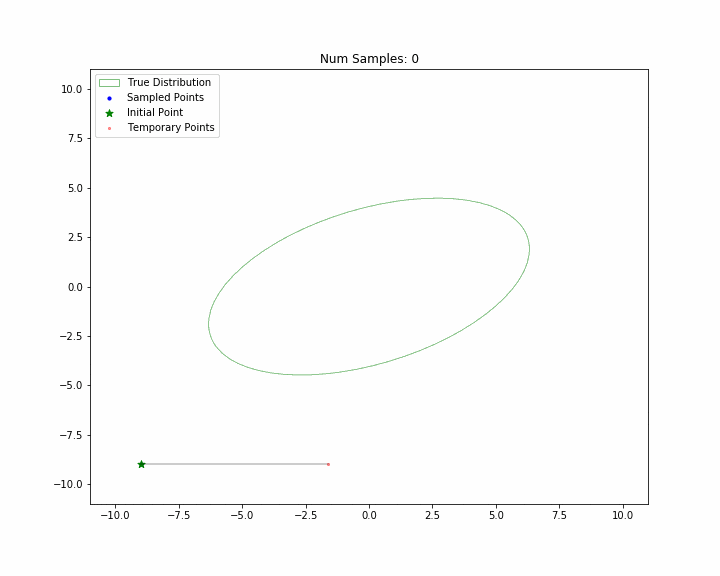
    return samples, tmp_points

Let’s see it in action. First let’s plot our true distribution, which lets say have the following parameters

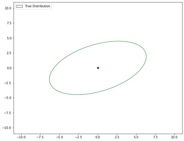
Let’s begin sampling! And also we will estimate a Gaussian from the sampled points to see how close we get to the true distribution with the increasing number of samples. Total number of sampled points = 500.

The complete code for this example along with all the plotting and creating GIFs is available at my github repository. For plotting Gaussian contours, I used the code from this matplotlib tutorial.

Now, of course, you won’t be using Gibbs sampling for sampling from multivariate Gaussians. So for any general intractable distribution, you need to have conditional samplers for each of the random variable given others. And you will be good to go.